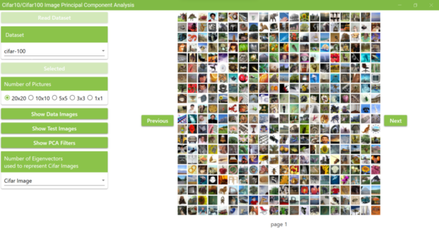
Principal Component Analysis of Cifar10/Cifar100 image datasets in C#
I wrote a program with Visual Studio 2022 to perform a principal component analysis of the Cifar10/Cifar100 image datasets using WPF, Material Design In XAML Toolkit, MahApps.Metro, Prism, and Accord.
The principal component vectors obtained by principal component analysis are converted to RGB values where the value of each vector element is from 0 to 255, and visualized as RGB images of size 32 x 32 pixels.
I also checked the representations of training data and test data by linear combinations of principal component vectors computed with Cifar10/Cifar100 training data. The number of principal component vectors arranged in order of decreasing eigenvalue was selected, and the training data and test data images were represented by linear combinations of the selected number of principal component vectors.
1. The source code has been placed at the following GitHub repository.
https://github.com/fukagai-takuya/cifar10-cifar100-principal-component-analysis/
I uploaded the executable files (MSIX package) for Windows 10 and Windows 11 on the following page.
## 2024.01.20: Although there is no change in the executable file, the program never crashed when I checked several times on Windows 11 Home 23H2 with the latest Windows Update applied.
https://www.leafwindow.com/softwares/msix/cifar10-cifar100-principal-component-analysis/
The procedure for installing the executable file is the same as this page.
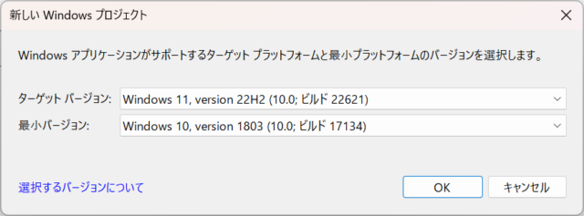
I confirmed that it works on Windows 11 Version 22H2. Since I specified Windows 10 Version 1803 to Windows 11 Version 22H2 as the target OS when creating the MSIX package, as shown in the attached image, it will work on Windows 10 Version 1803 or later.
2. About Cifar10/Cifar100 datasets
Cifar10 and Cifar100 are datasets of RGB images with 32 pixels height and 32 pixels width. Both Cifar10 and Cifar100 have a total of 60,000 images in the dataset. Among them, 50,000 images are training data used for learning weights of neural networks, and 10,000 images are test data used for evaluating image discrimination abilities of neural networks that have been trained.
The 60,000 images in Cifar10 show one of ten kinds of vehicles and creatures: airplane, automobile, bird, cat, deer, dog, frog, horse, ship, and truck. Each category has 6,000 images. These categories are given as labels for image data, which are used to train neural networks and evaluate their discrimination abilities.
The 60,000 images in Cifar100 contains 100 kinds of vehicles, creatures, electric appliances, etc. Each category has 600 images. 100 kinds of labels are assigned to Cifar100 images. The 100 labels are grouped into 20 groups. For example, beaver, dolphin, otter, seal, and whale are also assigned the group name, “aquatic mammals”.
3. About file structures of Cifar10/Cifar100 datasets (Binary version)
The following page is an explanation of Cifar10/Cifar100 datasets.
https://www.cs.toronto.edu/~kriz/cifar.html
3.1. The Cifar10 dataset, cifar-10-binary.tar.gz (Binary version), can be downloaded from the link below.
https://www.cs.toronto.edu/~kriz/cifar-10-binary.tar.gz
If you extract the compressed file cifar-10-binary.tar.gz with the following command,
$ tar xvzf cifar-10-binary.tar.gz
the following files will be extracted.
$ ls cifar-10-batches-bin
batches.meta.txt  data_batch_2.bin  data_batch_4.bin  readme.html
data_batch_1.bin  data_batch_3.bin  data_batch_5.bin  test_batch.bin
C:\dataset\tmp>where tar
C:\Windows\System32\tar.exe
C:\dataset\tmp>tar xvzf cifar-10-binary.tar.gz
x cifar-10-batches-bin/
x cifar-10-batches-bin/data_batch_1.bin
x cifar-10-batches-bin/batches.meta.txt
x cifar-10-batches-bin/data_batch_3.bin
x cifar-10-batches-bin/data_batch_4.bin
x cifar-10-batches-bin/test_batch.bin
x cifar-10-batches-bin/readme.html
x cifar-10-batches-bin/data_batch_5.bin
x cifar-10-batches-bin/data_batch_2.bin
3.2. The Cifar100 dataset, cifar-100-binary.tar.gz (Binary version), can be downloaded from the link below.
https://www.cs.toronto.edu/~kriz/cifar-100-binary.tar.gz
If you extract the compressed file cifar-100-binary.tar.gz with the following command,
$ tar xvzf cifar-100-binary.tar.gz
the following files will be extracted.
$ ls cifar-100-binary
fine_label_names.txt  coarse_label_names.txt  train.bin  test.bin
4. Contents of the Cifar10/Cifar100 datasets (Binary version) files
4.1. Contents of Cifar10 files
All of the following files are 30,730,000 bytes and contain 10,000 training images.
$ ls -l cifar-10-batches-bin/data_batch_*
-rw-r--r-- 1 fukagai 197610 30730000 Jun  5  2009 cifar-10-batches-bin/data_batch_1.bin
-rw-r--r-- 1 fukagai 197610 30730000 Jun  5  2009 cifar-10-batches-bin/data_batch_2.bin
-rw-r--r-- 1 fukagai 197610 30730000 Jun  5  2009 cifar-10-batches-bin/data_batch_3.bin
-rw-r--r-- 1 fukagai 197610 30730000 Jun  5  2009 cifar-10-batches-bin/data_batch_4.bin
-rw-r--r-- 1 fukagai 197610 30730000 Jun  5  2009 cifar-10-batches-bin/data_batch_5.bin
Like the files for training images, test_batch.bin, which stores test images, is 30,730,000 bytes and contains 10,000 test images.
$ ls -l cifar-10-batches-bin/test_batch.bin
-rw-r--r-- 1 fukagai 197610 30730000 Jun  5  2009 cifar-10-batches-bin/test_batch.bin
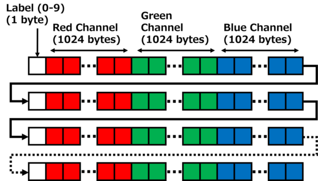
The first 1 byte of the 10,000 image data is the label number from 0 to 9, followed by 3,072 bytes of RGB image data. The image data is 3,072 bytes (1,024 x 3 = 3,072) consisting of 1,024 bytes of red data (32 x 32 = 1,024), 1,024 bytes of green data, and 1,024 bytes of blue data. The data is stored in the order shown in the figure below.
The batches.meta.txt contains the names corresponding to the label numbers from 0 to 9, as shown below. The names are listed in order of label number, with label number 0 being airplane, 1 being automobile, and 2 being bird.
airplane
automobile
bird
cat
deer
dog
frog
horse
ship
truck
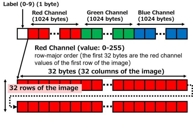
The 1,024 bytes of red data, 1,024 bytes of green data, and 1,024 bytes of blue data contain 32 x 32 pixels image data arranged in order from the first row.
The figure below is an example of red data. The first byte is the red value of the upper left corner pixel, and the first 32 bytes are the red values of the top row in the image. The 1,024th byte data at the end is the red value of the lower right corner pixel. Since it is 1 byte data, each value is an integer from 0 to 255. The same applies to green and blue data.
4.2. Contents of Cifar100 files
The data is structured similarly to the Cifar10 data, but the training data, train.bin is consisting of 50,000 images. test.bin is a file containing test data consisting of 10,000 images.
$ ls -l cifar-100-binary
-rw-r--r-- 1 fukagai 197610       328 Nov  3 12:22 coarse_label_names.txt
-rw-r--r-- 1 fukagai 197610       725 Nov  3 12:22 fine_label_names.txt
-rw-r--r-- 1 fukagai 197610  30740000 Nov  3 12:22 test.bin
-rw-r--r-- 1 fukagai 197610 153700000 Nov  3 12:22 train.bin
The composition of each image data is almost the same as that of Cifar10, but Cifar100 has two types of label numbers as shown in the figure below. The first byte, Coarse Label, is a label with a rough classification name such as aquatic_mammals. The Coarse Label value is from 0 to 19. The second byte, Fine Label, corresponds to beaver, dolphin, otter, seal, whale, etc. The Fine Label value is from 0 to 99.
The coarse_label_names.txt contains the names corresponding to the Coarse Label. The names are listed in order of the Coarse Label number, with label number 0 being aquatic_ammals, 1 being fish, and 2 being flowers.
aquatic_mammals
fish
flowers
food_containers
fruit_and_vegetables
...
The fine_label_names.txt contains the names corresponding to the Fine Label numbers. The names are listed in order of Fine Label number, with label number 0 being apple, 1 being aquarium_fish, and 2 being baby.
apple
aquarium_fish
baby
bear
beaver
...
5. How to read Cifar10/Cifar100 datasets and display images with this application.
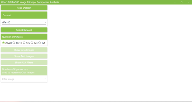
5.1. Immediately after the application is launched, the screen looks like this.
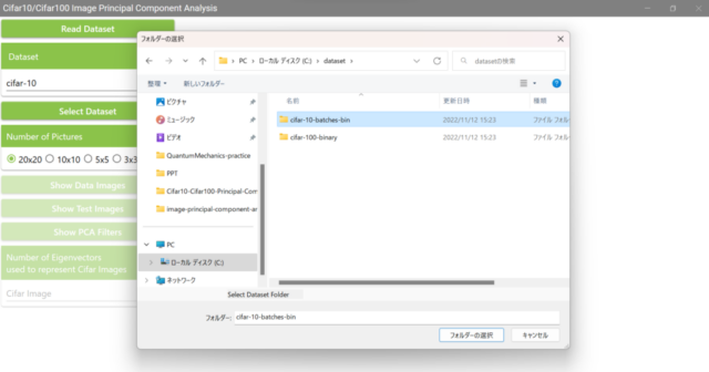
5.2. Click the Select Dataset button and select the Cifar10 folder you just extracted.
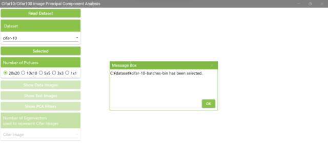
5.3. The following MessageBox will appear.
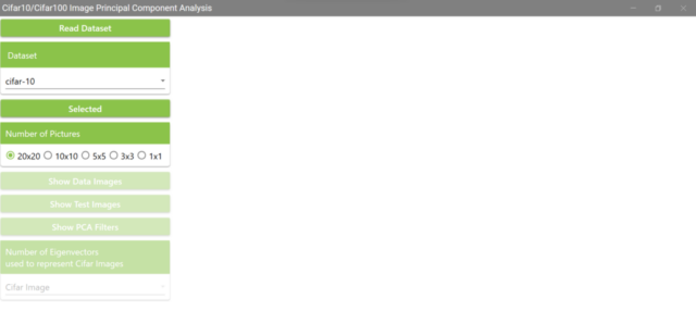
5.4. After selecting the dataset folder, you will see the following screen. Now click on the Read Dataset button to load the Cifar10 dataset.
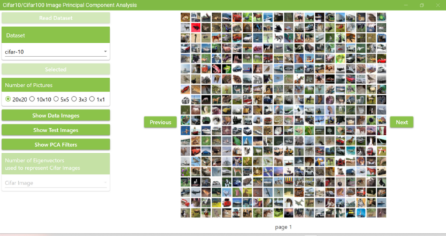
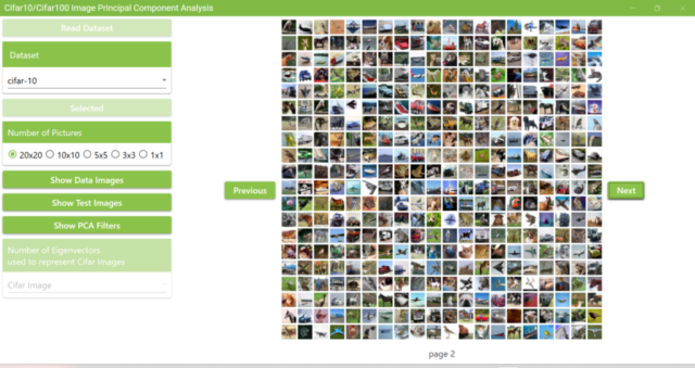
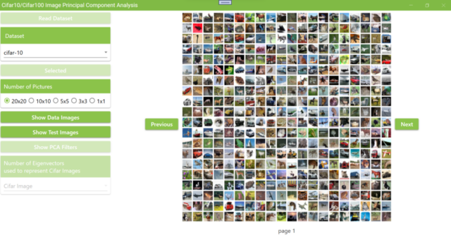
5.5. If the extracted Cifar10 dataset folder is selected, you will see the screen below. Image data from the Cifar10 dataset will be displayed.
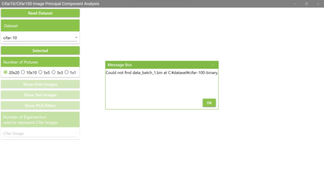
5.6. If you select a folder that does not have a Cifar10 dataset to load, a MessageBox will appear as shown below. In this example, the folder for the Cifar100 dataset was selected instead of the folder for the Cifar10 dataset, and the Cifar10 dataset failed to be loaded.
5.7. Click the Next and Previous buttons to view other images of Cifar10.
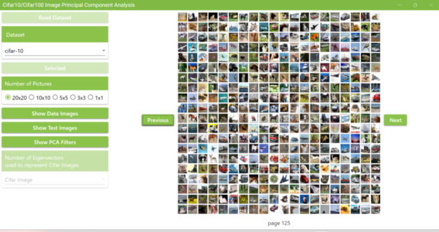
5.8. Cifar10 has 50,000 training data, so if I display 20×20 on each page, I will have 125 pages in total.
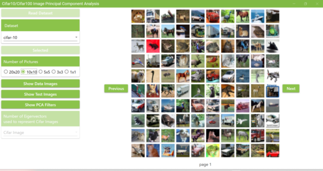
5.9. The number of images displayed on a page can be changed by clicking the Number of Pictures radio button. The example below shows a selection of 10×10.
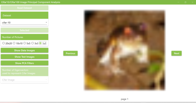
5.10. The image size of Cifar10 and Cifar100 are small, 32 pixels in height and 32 pixels in width, so if you select 1×1 in Number of Pictures and display only one image, you will see a slightly blurred image as shown in the figure below.
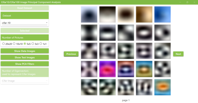
5.11. Next, click the Show PCA Filters button to display the PCA filters.
If you download and run the executable file linked below, you will immediately see the PCA filters. The pre-computed PCA filters are embedded in the executable file.
https://www.leafwindow.com/softwares/msix/cifar10-cifar100-principal-component-analysis/
If you build and run the source code at the link below, the first time you click the Show PCA Filters button, you will see a screen similar to the one shown below. The Show PCA Filters button fades and the PCA filters calculation begins.
https://github.com/fukagai-takuya/cifar10-cifar100-principal-component-analysis/
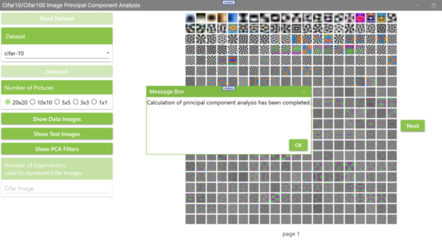
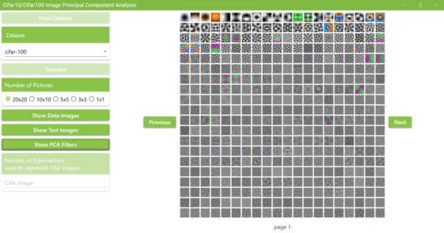
When the PCA filters calculation is complete, the Show PCA Filters button will return to its original color and a MessageBox will appear as shown below. It also displays images of the calculated PCA filters. The PCA filter images shown here are 32 x 32 pixels RGB images created by converting the principal component vector into RGB values ranging from 0 to 255. Principal component vectors are ordered starting with the first principal component. The principal component vectors are arranged from low to high frequency filters. The low-frequency filter shows a gradual change of RGB values in the image.
5.12. As with the Cifar10 images, click the Next and Previous buttons to see other PCA filters. The total number of PCA filter images obtained here is 3,072.
5.13. As with the Cifar10 images, the number of PCA filter images displayed at one time can be changed by clicking the Number of Pictures radio button.
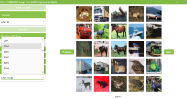
5.14. After clicking the Show Data Images button, change the selection of “Number of Eigenvectors used to represent Cifar Images” to represent Cifar10 images by superimposing PCA filters.
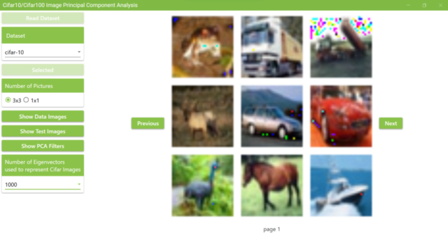
The example in the figure below attempts to represent Cidar10 training images by superimposing 1,000 PCA filters.
5.15. These images are the examples of superimposing 1,000 PCA filters to represent Cifar10 trainining images. Since this calculation is time consuming, only 3×3 or 1×1 images are displayed at a time. The images show fine dots that are not in the original images, but we can recognize which objects were displayed in the original images.
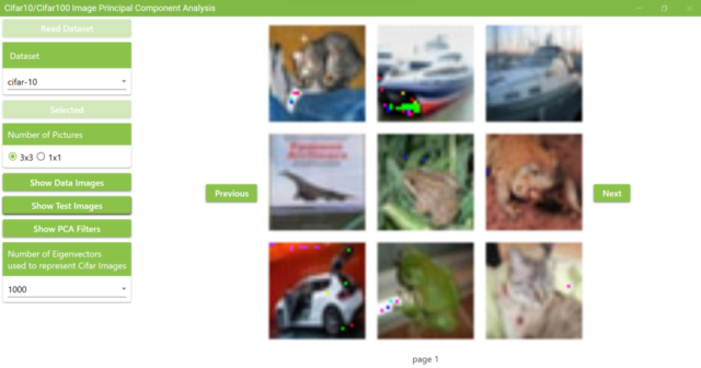
5.16. Now, clicking on the Show Test Images button will display images representing the test data by superimposing 1,000 PCA filters. The results are similar to the images representing training data by superimposing 1,000 PCA filters.
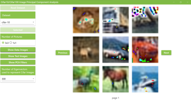
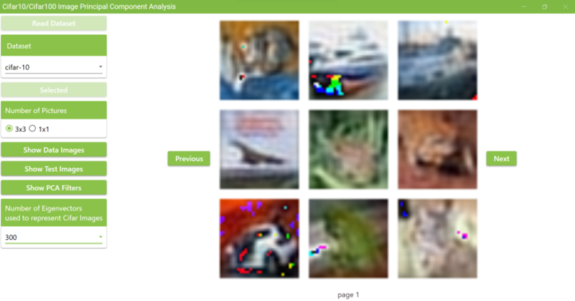
5.17. The figure below shows the results of changing the number of superimposed PCA filters to 300. Compared to the results of using 1,000 filters, it is harder to tell what are in the pictures.
a. Examples of displaying training data with 300 PCA filters
b. Examples of displaying test data with 300 PCA filters
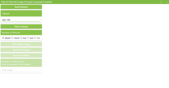
5.18. Changing the Dataset selection to Cifar100 will display similar results for Cifar100 data.
a. Immediately after switching the selection to Cifar100
b. Immediately after reading Cifar100 data
c. Results of clicking the PCA Filter button to display the PCA Filters
6. Principal Component Analysis for Cifar10/Cifar100 images
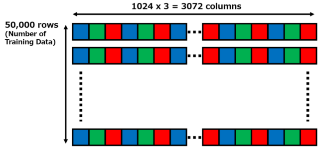
6.1. I prepared a matrix with 50,000 rows and 3,072 columns as shown in the figure below. Each line is the image data of Cifar10 or Cifar100 training data. From the pixel at the upper left corner to the pixel at the lower right corner, there are 3,072 bytes of data (32 x 32 = 1,024 pixels) arranged in B, G, R order. The training data is 50,000 rows of data since there are 50,000 training images.
6.2. In order to calculate principal component analysis, the matrix data in the above figure was stored in a two-dimensional array of type double, as shown in the code below, instead of type byte.
            double[,] X_input = new double[numberOfImages, ImageDataSize];
            for (int row = 0; row < numberOfImages; row++)
            {
                for (int column_i = 0; column_i < ImageAreaSize; column_i++)
                {
                    X_input[row, 3 * column_i] = (double) _dataImages[row].BlueChannelData[column_i]; // blue
                    X_input[row, 3 * column_i + 1] = (double) _dataImages[row].GreenChannelData[column_i]; // green
                    X_input[row, 3 * column_i + 2] = (double) _dataImages[row].RedChannelData[column_i]; // red
                }
            }
6.3. The principal component analysis was calculated using Accord.NET, which includes a C# matrix operations library, with the following code.
        private double[] _vectorMean;
        private double[,] _matrixU;
        private double[] _vectorW;
        private double[,] _matrixV;

        private void CalculatePCA()
        {
            ...

            // column means
            _vectorMean = X_input.Mean(dimension: 0);

            X_input = X_input.Subtract(_vectorMean, dimension: (VectorType)0);
            double[,] X_cov = X_input.Transpose().Dot(X_input);

            X_input = null;
            GC.Collect();

            SingularValueDecomposition svd = new SingularValueDecomposition(X_cov);

            _matrixU = svd.LeftSingularVectors;
            _vectorW = svd.Diagonal;
            _matrixV = svd.RightSingularVectors;

            ...
        }
6.4. The above calculation can be written in a mathematical formula as follows.
6.4.1. First, calculate the covariance matrix $X_{cov}$ of the RGB values for each pixel of the 50,000 training data using the following formula. The resulting covariance matrix $X_{cov}$ is a 3,072-by-3,072 matrix. Since dividing or not dividing the entire obtained result by 50,000 or 49,999 does not affect the principal component vectors, I use the following result as the covariance matrix $X_{cov}$. This is because whether or not the entire covariance matrix is multiplied by a constant does not affect the direction of the principal component vectors that I want to calculate this time.
\[X_{cov} = (X_{input} – X_{mean})^T (X_{input} – X_{mean})\]
In the above formula, $X_{input}$ is the image data of 50,000 rows and 3,072 columns, and $X_{mean}$ is the mean value matrix of 50,000 rows and 3,072 columns that stores the mean value of each column in $X_{input}$.
$X_{mean}$ is a matrix that stores the mean of the RGB values at each pixel of 50,000 images. Each column of $X_{mean}$ contains the same value. The first column of $X_{mean}$ contains the mean value of the blue component (B) at the upper left corner. The same values are lined up from row 1 to row 50,000. The mean of the RGB component of each pixel in the training data for Cifar10 and Cifar100 was around 120 to 140.
$(X_{input} – X_{mean})^T$ is a 3,072-by-50,000 matrix with the mean subtracted and transposed. The diagonal components of the 3,072-by-3,072 covariance matrix $X_{cov}$ obtained by the above calculation are the variances of the RGB values at each pixel position. Except for the diagonal component, the covariance is the covariance of the image data calculated by taking two locations from the 3,072 RGB values.
6.4.2. Next, $X_{cov}$ is decomposed into singular values as in the following equation.
\[X_{cov} = UWV\]
The $U$, $W$, and $V$ in the above equation are all 3,072-by-3,072 matrices, with $W$ being a diagonal matrix and $U$ and $V$ being orthogonal matrices. The singular value decomposition of the covariance matrix yields $V=U^T$, where $UV$ is the unit matrix.
Using Accord.NET’s Singular Value Decomposition class SingularValueDecomposition, the diagonal matrix $W$ yields a result in which the numbers are arranged in descending order from largest value to smallest in the diagonal components. In the previous code _vectorW = svd.Diagonal, only the diagonal components of the diagonal matrix are obtained as a vector of 3,072 elements.
Also, what you get with _matrixV = svd.RightSingularVectors is $V^T$, that is the transposed matrix of $V$ in the above equation. The following calculations are performed to confirm that the unit matrix is obtained.
double[,] UV = _matrixU.Transpose().Dot(_matrixV);
| processor | Intel(R) Core(TM) i3-8145U CPU @ 2.10GHz 2.30 GHz |
| RAM | 8.00 GB (7.75 GB available) |
| System type | 64-bit operating system, x64-based processor |
| edition | Windows 11 Home |
| version | 22H2 |
| OS Build | 22621.819 |
| Matrix Calculation Package | Accord.Math 3.8.0 |
